Data
The data looks a bit irregular in the beginning of the curves, but seems well behaving nonetheless.
IV <- data.frame(
time=c(0.33,0.5,0.67,1.5,2,4,6,10,16,24,32,48),
conc=c(14.7,12.6,11,9,8.2,7.9,6.6,6.2,4.6,3.2,2.3,1.2))
Oral <- data.frame(
time=c(0.5,1,1.5,2,4,6,10,16,24,32,48),
conc=c(2.4,3.8,4.2,4.6,8.1,5.8,5.1,4.1,3,2.3,1.3))
plot(conc~time,data=IV[1:12,],log='y',col='blue',type='l')
with(Oral,lines(y=conc,x=time,col='red'))

Jags model
A n umber of questions are asked. It is the intention the model gives posteriors for all. Priors are on clearance, volume and a few other variables. The increasing part of the oral curve is modeled with a second compartment. The same is true for the sharp decreasing part of the IV model. However, where the increasing part is integral part of the PK calculations, the decreasing part of IV is subsequently ignored. I have been thinking of removing these first points, but in the end rather than using personal judgement I just modeled them so I could ignore them afterwards.
library(R2jags)
datain <- list(
timeIV=IV$time,
concIV=IV$conc,
nIV=nrow(IV),
doseIV=500,
timeO=Oral$time,
concO=Oral$conc,
nO=nrow(Oral),
doseO=500)
model1 <- function() {
tau <- 1/pow(sigma,2)
sigma ~ dunif(0,100)
# IV part
kIV ~dnorm(.4,1)
cIV ~ dlnorm(1,.01)
for (i in 1:nIV) {
predIV[i] <- c0*exp(-k*timeIV[i]) +cIV*exp(-kIV*timeIV[i])
concIV[i] ~ dnorm(predIV[i],tau)
}
c0 <- doseIV/V
V ~ dlnorm(2,.01)
k <- CL/V
CL ~ dlnorm(1,.01)
AUCIV <- doseIV/CL+cIV/kIV
# oral part
for (i in 1:nO) {
predO[i] <- c0star*(exp(-k*timeO[i])-exp(-ka*timeO[i]))
concO[i] ~ dnorm(predO[i],tau)
}
c0star <- doseO*(ka/(ka-k))*F/V
AUCO <- c0star/k
F ~ dunif(0,1)
ka ~dnorm(.4,1)
ta0_5 <- log(2) /ka
t0_5 <- log(2)/k
}
parameters <- c('k','AUCIV','CL','V','t0_5','c0',
'AUCO','F','ta0_5','ka','c0star',
'kIV','cIV','predIV','predO')
inits <- function()
list(
sigma=rnorm(1,1,.1),
V=rnorm(1,25,1),
kIV=rnorm(1,1,.1),
cIV = rnorm(1,10,1),
CL = rnorm(1,5,.5),
F = runif(1,0.8,1),
ka = rnorm(1,1,.1)
)
jagsfit <- jags(datain, model=model1,
inits=inits, parameters=parameters,progress.bar="gui",
n.chains=4,n.iter=14000,n.burnin=5000,n.thin=2)
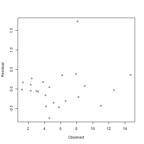
Quality of fit
A plot of the posterior fit against the original data. It would seem we have an outlier.
cin <- c(IV$conc,Oral$conc)
mIV <- sapply(1:ncol(jagsfit$BUGSoutput$sims.list$predIV),
function(x) {
mean(jagsfit$BUGSoutput$sims.list$predIV[,x])
}
)
mO <- sapply(1:ncol(jagsfit$BUGSoutput$sims.list$predO),
function(x) {
mean(jagsfit$BUGSoutput$sims.list$predO[,x])
}
)
plot(x=c(IV$conc,Oral$conc),y=c(IV$conc,Oral$conc)-c(mIV,mO))
Answers to questions
We have the following posteriors:
Inference for Bugs model at "C:/...BEnL/model1b6027171a7a.txt", fit using jags,
4 chains, each with 14000 iterations (first 5000 discarded), n.thin = 2
n.sims = 18000 iterations saved
mu.vect sd.vect 2.5% 25% 50% 75% 97.5% Rhat n.eff
AUCIV 219.959 16.975 189.743 208.636 218.846 230.210 256.836 1.002 2800
AUCO 200.468 15.102 171.908 190.523 199.987 209.928 231.722 1.001 7500
CL 2.346 0.182 1.995 2.226 2.344 2.461 2.712 1.002 2900
F 0.876 0.052 0.773 0.841 0.876 0.911 0.976 1.002 3200
V 56.463 2.752 51.610 54.583 56.280 58.112 62.465 1.002 3100
c0 8.876 0.426 8.005 8.604 8.884 9.160 9.688 1.002 3100
c0star 8.314 0.615 7.119 7.911 8.304 8.704 9.574 1.002 2000
cIV 11.229 2.485 7.029 9.511 11.003 12.654 16.804 1.003 1100
k 0.042 0.004 0.034 0.039 0.042 0.044 0.050 1.002 2200
kIV 2.064 0.510 1.132 1.704 2.041 2.396 3.126 1.004 800
ka 0.659 0.105 0.489 0.589 0.646 0.715 0.903 1.002 3200
predIV[1] 14.343 0.532 13.240 14.009 14.355 14.690 15.378 1.002 2500
predIV[2] 12.637 0.331 11.990 12.422 12.632 12.851 13.298 1.001 12000
predIV[3] 11.435 0.357 10.755 11.196 11.427 11.667 12.147 1.002 1600
predIV[4] 8.923 0.326 8.333 8.709 8.902 9.116 9.638 1.002 2900
predIV[5] 8.410 0.298 7.845 8.213 8.401 8.594 9.021 1.001 14000
predIV[6] 7.522 0.286 6.943 7.340 7.525 7.713 8.064 1.001 5900
predIV[7] 6.910 0.255 6.385 6.749 6.915 7.077 7.399 1.001 6200
predIV[8] 5.848 0.222 5.406 5.704 5.849 5.993 6.285 1.001 7800
predIV[9] 4.557 0.231 4.098 4.409 4.555 4.707 5.012 1.001 4500
predIV[10] 3.270 0.252 2.781 3.107 3.267 3.433 3.773 1.002 3100
predIV[11] 2.349 0.251 1.867 2.183 2.343 2.509 2.865 1.002 2700
predIV[12] 1.217 0.207 0.839 1.076 1.204 1.343 1.662 1.002 2500
predO[1] 2.138 0.214 1.750 1.995 2.124 2.263 2.599 1.001 8700
predO[2] 3.626 0.293 3.070 3.432 3.616 3.807 4.234 1.001 12000
predO[3] 4.653 0.306 4.050 4.452 4.652 4.847 5.264 1.001 16000
predO[4] 5.351 0.294 4.754 5.161 5.354 5.541 5.930 1.001 15000
predO[5] 6.375 0.277 5.801 6.202 6.383 6.562 6.894 1.002 3200
predO[6] 6.274 0.308 5.629 6.079 6.286 6.485 6.842 1.002 2800
predO[7] 5.455 0.292 4.852 5.270 5.461 5.648 6.018 1.002 3900
predO[8] 4.262 0.245 3.764 4.106 4.265 4.423 4.736 1.001 8600
predO[9] 3.057 0.227 2.605 2.910 3.058 3.207 3.504 1.001 8200
predO[10] 2.195 0.218 1.773 2.050 2.192 2.335 2.638 1.001 5200
predO[11] 1.135 0.180 0.805 1.013 1.127 1.247 1.519 1.002 3500
t0_5 16.798 1.713 13.830 15.655 16.652 17.770 20.617 1.002 2200
ta0_5 1.077 0.164 0.768 0.969 1.072 1.177 1.419 1.002 3200
deviance 38.082 5.042 30.832 34.357 37.207 40.918 50.060 1.003 1200
For each parameter, n.eff is a crude measure of effective sample size,
and Rhat is the potential scale reduction factor (at convergence, Rhat=1).
DIC info (using the rule, pD = var(deviance)/2)
pD = 12.7 and DIC = 50.8
DIC is an estimate of expected predictive error (lower deviance is better).
Expected answers:
t1/2=16.7 hr, AUCiv=217 mg-hr/L, AUCoral=191 mg-hr/L, CL=2.3 L/hr, V=55L, F=0.88While the point estimates are close, the s.d. seem quite large.
Plot of models
A plot of the predicted concentration time curves, with confidence intervals. The wider intervals at the low end of the concentrations are due to the logarithmic scale.
tpred <- 0:48
simO <- sapply(1:jagsfit$BUGSoutput$n.sims,function(x) {
jagsfit$BUGSoutput$sims.list$c0star[x]*
(exp(-jagsfit$BUGSoutput$sims.list$k[x]*tpred)
-exp(-jagsfit$BUGSoutput$sims.list$ka[x]*tpred))
})
predO <- data.frame(mean=rowMeans(simO),sd=apply(simO,1,sd))
simIV <- sapply(1:jagsfit$BUGSoutput$n.sims,function(x) {
jagsfit$BUGSoutput$sims.list$c0[x]*
(exp(-jagsfit$BUGSoutput$sims.list$k[x]*tpred)
+exp(-jagsfit$BUGSoutput$sims.list$kIV[x]*tpred))
})
predIV <- data.frame(mean=rowMeans(simIV),sd=apply(simIV,1,sd))
plot(conc~time,data=IV[1:12,],log='y',col='blue',type='p',ylab='Concentration')
with(Oral,points(y=conc,x=time,col='red'))
lines(y=predO$mean,x=tpred,col='red',lty=1)
lines(y=predO$mean+1.96*predO$sd,x=tpred,col='red',lty=2)
lines(y=predO$mean-1.96*predO$sd,x=tpred,col='red',lty=2)
lines(y=predIV$mean,x=tpred,col='blue',lty=1)
lines(y=predIV$mean+1.96*predIV$sd,x=tpred,col='blue',lty=2)
lines(y=predIV$mean-1.96*predIV$sd,x=tpred,col='blue',lty=2)

Nice post!
ReplyDeleteI translated your model and data to Stan format, fit it, and posted the results on Gelman's blog, in the post Stan Model of the Week: PK Calculation of IV and Oral Dosing. Oddly, the results are a bit different, though both contain your reported "correct" values in their posterior 95% intervals.
Andrew, Daniel Lee, and I have been working with Frederic Bois on adding ODE solvers to Stan (along the lines of PKBUGS), so we've been thinking about PK/PD models a lot lately.
I had mistranslated the lognormal priors as normal; with that fix, Stan and JAGS produce the same results.
DeleteWingfeet,
ReplyDeleteCan you comment how did you choose pretty informative log normal priors? Why priors for kIV and ka are normal - and quite tight?
Thank you
Hi Linas,
DeleteThat is a good question. These priors even allow negative k, which on consideration I think is fairly strange. Probably these should have been log normal. dlnorm(.4,.1) seems a much better choice.