Sunday, December 28, 2014

A time series contest attempt

I saw the post a time series contest on Rob J Hyndman's blog. Since I am still wanting to play around with some bigger data sets, so I went to the source website https://drive.google.com/folderview?id=0BxmzB6Xm7Ga1MGxsdlMxbGllZnM&usp=sharing and got myself the data. One warning, if you are reading this to know how to get close to the winning result, you'd better stop now. I did not get even close.

Data

Data exists in two data sets, training and test. The data are time series, each of a 1000 time points and some summary statistics of these. The training set consists of 63530 samples, the test set an additional 77769. In practice this means 490 Mb and 600 Mb of memory. Not surprising, just prepping the data and dropping it in randomForest gives an out of memory error. The question then is how to preserve memory.
It seemed that my Windows 7 setup used more memory than my Suse 13.2 setup. The latter is quite fresh, while Win 7 has been used two years now, so there may be some useless crap which wants to be resident there. I did find that Chrome keeps part of itself resident, so switched that off (advanced setting). Other things which Win 7 has and Suse 13.2 misses are Google drive (it cannot be that hard to make it, but Google is dragging its heels) and a virus scanner, but there may be more.
This helped a bit, but this data gave me good reason to play a bit with dplyr's approach to store data in a database.
library(dplyr)
library(randomForest)
library(moments)

load('LATEST_0.2-TRAIN_SAMPLES-NEW_32_1000.saved')
my_db <- src_sqlite(path = tempfile(), create = TRUE)
#train_samples$class <- factor(train_samples$class)
train_samples$rowno <- 1:nrow(train_samples)
train <- copy_to(my_db,train_samples,indexes=list('rowno'))
rm(train_samples)

So, the code above reads the data and stores it in a SQLite database. At one point I made class a factor, but since SQLite does not have factors, this property is removed once the data is retrieved out of the database. I added a rowno variable. Some database engines have a function for row numbers, SQLite does not, and I need it to select records.
The key learning I got from this is related to the rowno variable. Once data is in the database, it just knows what is in the database and only understands its own flavour of SQL. Dplyr does a good job to make it as similar as possible to data.frames, but in the end one needs to have a basic understanding of SQL to get it to work.

Plot

The data has the property that part of it, the last n time points, are true samples. In this part the samples have an increase or decrease of 0.5%. The question is then what happens in the next part, further increase or decrease. The plot below shows the true samples of the first nine records. What is not obvious from the figure, is that the first two records have the same data, except for a different true part.  

First model

As a first step I tried a model with limited variables and only 10000 records. For this the x data has been compressed in two manners. From a time series perspective, where the ACF is used, and from trend perspective, where 10 points are used to capture general shape of the curves. The latter by using local regression (loess). Both these approaches are done on true data and all data. In addition, the summary variables provided in the data are used.
The result, an OOB error rate of 44%. Actually, this was a lucky run, I have had runs with error rates over 50%. I did not bother to check predictive capability.
mysel <- filter(train,rowno<10000) %>%
        select(.,-chart_length,-rowno) %>%
        collect()
yy <- factor(mysel$class)
vars <- as.matrix(select(mysel,var.1:var.1000))
leftp <- select(mysel,true_length:high_frq_true_samples)
rm(mysel)
myacf <- function(datain) {
    a1 <- acf(datain$y,plot=FALSE,lag.max=15)
    a1$acf[c(2,6,11,16),1,1]
}
myint <- function(datain) {
    ll <- loess(y ~x,data=datain)
    predict(ll,data.frame(x=seq(0,1,length.out=10)))
}

la <- lapply(1:nrow(vars),function(i) {
            allvar <- data.frame(x=seq(0,1,length.out=1000),y=vars[i,])
            usevar <- data.frame(x=seq(0,1,length.out=leftp$true_length[i]),
                    y=allvar$y[(1001-leftp$true_length[i]):1000])
            c(myacf(allvar),myacf(usevar),myint(allvar),myint(usevar))
        })
rm(vars)
rightp <- do.call(rbind,la)
colnames(rightp) <- c(
        paste('aacf',c(2,6,11,16),sep=''),
        paste('uacf',c(2,6,11,16),sep=''),
        paste('a',seq(1,10),sep=''),
        paste('u',seq(1,10),sep=''))

xblok <- as.matrix(cbind(leftp,rightp))
rf1 <-randomForest(
        x=xblok,
        y=yy,
        importance=TRUE)
rf1

Call:
 randomForest(x = xblok, y = yy, importance = TRUE)
               Type of random forest: classification
                     Number of trees: 500
No. of variables tried at each split: 6

        OOB estimate of  error rate: 44.21%
Confusion matrix:
     0    1 class.error
0 2291 2496   0.5214122
1 1925 3287   0.3693400

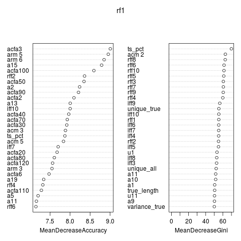
The plot shows the variable importance. Besides the variables provided the ACF seems important. Variables based on all time points seemed to work better than variables based on the true time series.

Second Model

In this model extra detail has been added to the all data variables. In addition extra momemnts of the data have been calculated. It did not help very much.
mysel <- filter(train,rowno<10000) %>%
        select(.,-chart_length,-rowno) %>%
        collect()
yy <- factor(mysel$class)
vars <- as.matrix(select(mysel,var.1:var.1000))
leftp <- select(mysel,true_length:high_frq_true_samples)
rm(mysel)
myacf <- function(datain,cc,lags) {
    a1 <- acf(datain$y,plot=FALSE,lag.max=max(lags)-1)
    a1 <- a1$acf[lags,1,1]
    names(a1) <- paste('acf',cc,lags,sep='')
    a1
}
myint <- function(datain,cc) {
    datain$y <- datain$y/mean(datain$y)
    ll <- loess(y ~x,data=datain)
    pp <- predict(ll,data.frame(x=seq(0,1,length.out=20)))
    names(pp) <- paste(cc,1:20,sep='')
    pp
}

la <- lapply(1:nrow(vars),function(i) {
            allvar <- data.frame(x=seq(0,1,length.out=1000),y=vars[i,])
            usevar <- data.frame(x=seq(0,1,length.out=leftp$true_length[i]),
                    y=allvar$y[(1001-leftp$true_length[i]):1000])
            acm <- all.moments(allvar$y,central=TRUE,order.max=5)[-1]
            names(acm) <- paste('acm',2:6)
            arm <- all.moments(allvar$y/mean(allvar$y),
                    central=FALSE,order.max=5)[-1]
            names(arm) <- paste('arm',2:6)
            ucm <- all.moments(usevar$y,central=TRUE,order.max=5)[-1]
            names(ucm) <- paste('ucm',2:6)
            urm <- all.moments(usevar$y/mean(usevar$y),
                    central=FALSE,order.max=5)[-1]
            names(urm) <- paste('urm',2:6)       
            ff <- fft(allvar$y[(1000-511):1000])[1:10]
            ff[is.na(ff)] <- 0
            rff <- Re(ff)
            iff <- Im(ff)
            names(rff) <- paste('rff',1:10,sep='')
            names(iff) <- paste('iff',1:10,sep='')
            c(myacf(allvar,'a',lags=c(2:10,seq(20,140,by=10))),
                    myint(allvar,'a'),
                    acm,
                    arm,
                    rff,
                    iff,
                    myacf(usevar,'u',seq(2,16,2)),
                    myint(usevar,'u')
            )
        })
#rm(vars)
rightp <- do.call(rbind,la)
xblok <- as.matrix(cbind(leftp,rightp))
rf1 <-randomForest(
        x=xblok,
        y=yy,
        importance=TRUE,
        nodesize=5)
rf1

Call:
 randomForest(x = xblok, y = yy, importance = TRUE)
               Type of random forest: classification
                     Number of trees: 500
No. of variables tried at each split: 10

        OOB estimate of  error rate: 42.76%
Confusion matrix:
     0    1 class.error
0 2245 2542   0.5310215
1 1734 3478   0.3326938


SVM

Just to try something else than a randomForest. But I notice some overfitting.
sv1 <- svm(x=xblok,
        y=yy
        )
sv1
Call:
svm.default(x = xblok, y = yy)

Parameters:
   SVM-Type:  C-classification
 SVM-Kernel:  radial
       cost:  1
      gamma:  0.009259259

Number of Support Vectors:  9998
table(predict(sv1),yy)

   yy
       0    1
  0 4776    2
  1   11 5210

A test set (rowno>50000 in the training table) did much worse
   ytest
       0    1
  0  547  580
  1 6254 6149

Sunday, December 21, 2014

Merry Christmas

Based on The DO loop, since I wanted a fractal Christmas tree and there is no point in inventing what has been made already. Besides, this is not the first time this year that I used R to do what has been done in SAS.

Code

# http://blogs.sas.com/content/iml/2012/12/14/a-fractal-christmas-tree/
# Each row is a 2x2 linear transformation 
# Christmas tree 
L <-  matrix(
    c(0.03,  0,     0  ,  0.1,
        0.85,  0.00,  0.00, 0.85,
        0.8,   0.00,  0.00, 0.8,
        0.2,  -0.08,  0.15, 0.22,
        -0.2,   0.08,  0.15, 0.22,
        0.25, -0.1,   0.12, 0.25,
        -0.2,   0.1,   0.12, 0.2),
    nrow=4)
# ... and each row is a translation vector
B <- matrix(
    c(0, 0,
        0, 1.5,
        0, 1.5,
        0, 0.85,
        0, 0.85,
        0, 0.3,
        0, 0.4),
    nrow=2)

prob = c(0.02, 0.6,.08, 0.07, 0.07, 0.07, 0.07)

# Iterate the discrete stochastic map 
N = 1e5 #5  #   number of iterations 
x = matrix(NA,nrow=2,ncol=N)
x[,1] = c(0,2)   # initial point
k <- sample(1:7,N,prob,replace=TRUE) # values 1-7 

for (i in 2:N) 
  x[,i] = crossprod(matrix(L[,k[i]],nrow=2),x[,i-1]) + B[,k[i]] # iterate 

# Plot the iteration history 
png('card.png')
par(bg='darkblue',mar=rep(0,4))    
plot(x=x[1,],y=x[2,],
    col=grep('green',colors(),value=TRUE),
    axes=FALSE,
    cex=.1,
    xlab='',
    ylab='' )#,pch='.')

bals <- sample(N,20)
points(x=x[1,bals],y=x[2,bals]-.1,
    col=c('red','blue','yellow','orange'),
    cex=2,
    pch=19
)
text(x=-.7,y=8,
    labels='Merry',
    adj=c(.5,.5),
    srt=45,
    vfont=c('script','plain'),
    cex=3,
    col='gold'
)
text(x=0.7,y=8,
    labels='Christmas',
    adj=c(.5,.5),
    srt=-45,
    vfont=c('script','plain'),
    cex=3,
    col='gold'
)

Sunday, December 14, 2014

Monthly Weather in Netherlands

When I downloaded the KNMI meteorological data, the intention was to do something which takes more than just the computers memory. While it is clearly not big data, at the very least 100 years of daily data is not small either. So I took along a load of extra variables to see what trouble I would run into. I did not run out of memory, but did make some figures.

Data

Data are acquired from KNMI. They have various sets of data, this page has a selection form which leads to the data used today. The data comes with a header explaining details, unfortunately in Dutch.

Plots

Just about everybody knows days are shorter in winter. What I never realized, even within that shorter day, we get less daylight. The short days are often so clouded, we don't get sun, meanwhile, in summer the sun does shine a bigger part of the daylight period.


In real hours sunshine this results in the following plot. December clearly has the darkest hours.
What we do get, not surprising since Dutch weather is fairly similar to English weather, is rain. Not continuous rain, most of the time it is dry, but still, autumn and winter do have days where it does not seem to stop. Autumn has the bad reputation for rain, but this plot makes winter look particular bad.
All this rain gives a load of humidity. This humidity in its turn, gives rise to a weather we name 'waterkoud'. It is above zero C but still quite cold outside. The humidity makes for air with a high heat capacity, hence one cools down quickly. Temperatures below zero can make for much nicer weather, but that can hamper traffic quite a lot. Most of the time it just doesn't freeze.
Code

library(plyr)
library(dplyr)
library(ggplot2)
r1 <- read.csv('KNMI_20141115.edited.txt')
Sys.setlocale(category = "LC_TIME", locale = "C")
r2 <- mutate(r1,
    date = as.Date(format(YYYYMMDD),'%Y%m%d'),
    month =factor(months(date,abbreviate=TRUE),
        levels=months(as.Date(
                paste('2014',
                    formatC(1:12,digits=2,width=2,flag='0'),
                    '01',sep='-')),
            abbreviate=TRUE)),
    yearf=factor(format(date,'%Y')),
    yearn=as.numeric(substr(YYYYMMDD,1,4)),
    day=format(date,'%e'))

g1 <- ggplot(r2,aes(x=month,y=SP))
g1 + geom_violin() +
        ylab('% of longest possible sunshine')

g1 <- ggplot(r2,aes(x=month,y=SQ/10))
g1 + geom_violin()  +
        ylab('Sunshine duration (h)')

g1 <- ggplot(r2,aes(x=month,y=DR/10))
g1 + geom_violin() +
        scale_y_continuous('Precipitation Duration (h)',
                breaks=c(0,6,12,18,24))

g1 <- ggplot(r2,aes(x=month,y=UG))
g1 + geom_violin() +
        ylab('Relative Humidity (%)')
 

g1 <- ggplot(r2,aes(x=month,y=TG/10))
g1 + geom_violin() +
        ylab('Temperature (C)')

Saturday, December 6, 2014

SAS PROC MCMC in R: Nonlinear Poisson Regression Models

In exercise 61.1 the problem is that the model has bad mixing. In the SAS manual the mixing is demonstrated after which a modified distribution is used to fix the model.
In this post the same problem is tackled in R; MCMCpack, RJags, RStan and LaplaceDemon. MCMCpack has quite some mixing problems, RStan seems to do best.

Data

To quote the SAS manual "This example shows how to analyze count data for calls to a technical support help line in the weeks immediately following a product release. (...) You can model the number of daily calls as a Poisson random variable, with the average number of calls modeled as a nonlinear function of the number of weeks that have elapsed since the product’s release. (...) During the first several weeks after a new product is released, the number of questions that technical support receives concerning the product increases in a sigmoidal fashion. The expression for the mean value in the classic Poisson regression involves the log link. There is some theoretical justification for this link, but with MCMC methodologies, you are not constrained to exploring only models that are computationally convenient. The number of calls to technical support tapers off after the initial release, so in this example you can use a logistic-type function to model the mean number of calls received weekly for the time period immediately following the initial release."
observed <- scan(text='
1 0 1 2 2 2 2 1 3 1 3 3
4 5 4 8 5 5 5 9 6 17 6 9
7 24 7 16 8 23 8 27',
    what=list(integer(),integer()),
    sep=' ',
)
names(observed) <- c('weeks','calls')
observed <- as.data.frame(observed)

Analysis

MCMCpack

The MCMCpack solution is derived from LaplacesDemon solution below. It is placed as first because it shows some of the problems with the mixing. As a change from LaplacesDemon, gamma could get negative, for which I made a -Inf likelihood.
library(MCMCpack)
MCMCfun <- function(parm) {
    names(parm) <- c('alpha','beta','gamma')
    if (parm['gamma']<0) return(-Inf)
    mu <-parm['gamma']*
        LaplacesDemon::invlogit(parm['alpha']+parm['beta']*observed$weeks)
    LL <- sum(dpois(observed$calls,mu,log=TRUE))
    LP <- LL+ dgamma(parm['gamma'],shape=3.4,scale=12,log=TRUE) +
        dnorm(parm['alpha'],-5,sd=.25,log=TRUE) +
        dnorm(parm['beta'],0.75,.5,log=TRUE)
    return(LP)
}
mcmcout <- MCMCmetrop1R(MCMCfun,
    c(alpha=-4,beta=1,gamma=2))

The figures show bad mixing. Parameters, especially Beta and Gamma, get stuck. There is quite some autocorrelation.
plot(mcmcout)
acf(mcmcout)
The cause is a nasty correlation between Beta and Gamma
pairs(as.data.frame(mcmcout))

LaplacesDemon

I chose an adaptive algorithm for LaplacesDemon. For the specs, the numbers are derived from the standard deviation of a previous run. Stepsize keeps reasonably constant through the latter part of run. The samples look much better than MCMCpack, although the mixing is not ideal either.
At a later stage I tried this same analysis with reflective Slice Sampler, however, that did was quite a bit more difficult and the end result was not better than this.
library('LaplacesDemon')
mon.names <- "LP"
parm.names <- c('alpha','beta','gamma')
PGF <- function(Data) c(rnorm(3,0,1))
N <-1
MyData <- list(mon.names=mon.names,
    parm.names=parm.names,
    PGF=PGF,
    calls=observed$calls,
    weeks=observed$weeks)
Model <- function(parm, Data)
{
    mu <-parm['gamma']*
        invlogit(parm['alpha']+parm['beta']*Data$weeks)
    LL <- sum(dpois(Data$calls,mu,log=TRUE))
    LP <- LL+ dgamma(parm['gamma'],shape=3.4,scale=12,log=TRUE) +
        dnorm(parm['alpha'],-5,sd=.25,log=TRUE) +
        dnorm(parm['beta'],0.75,.5,log=TRUE)
    Modelout <- list(LP=LP, Dev=-2*LL, Monitor=LP,
        yhat=mu,
        parm=parm)
    return(Modelout)
}

Initial.Values <- c(alpha=-4,beta=1,gamma=2) #GIV(Model, MyData, PGF=TRUE)
Fit1 <- LaplacesDemon(Model,
    Data=MyData,
    Initial.Values = Initial.Values,
    Algorithm = "AHMC",
    Specs = list(epsilon = c(.23,.2,13.5)/4,
        L = 2, Periodicity = 10),
    Iterations=40000,Status=2000   
)
BurnIn <- Fit1$Rec.BurnIn.Thinned
plot(Fit1, BurnIn, MyData, PDF=FALSE)

Jags

I do not think using one chain is advisable, especially since Jags makes more chains so easy. But in the spirit of this analysis I am using one. Coda plots are used since they are a bit more compact.
library(R2jags)
datain <- list(
    calls=observed$calls,
    weeks=observed$weeks,
    n=nrow(observed))
parameters <- c('alpha','beta','gamma')

jmodel <- function() {
    for (i in 1:n) {       
        mu[i] <- gamma*ilogit(alpha+beta*weeks[i])
        calls[i] ~ dpois(mu[i])
    }
    alpha ~ dnorm(-5,1/(.25*.25))
    gamma ~ dgamma(3.4,1/12)
    beta ~ dnorm(.75,1/(.5*.5))
}

jj <- jags(model.file=jmodel,
    data=datain,
    parameters=parameters,
    n.chains=1,
    inits=list(list(alpha=-4,beta=1,gamma=2))
    )

cc <- as.mcmc(jj$BUGSoutput$sims.array[,1,])

plot(cc)
acfplot(cc)

Stan

Stan probably does best handling this typical distribution. Again, one chain is only in the context of this posting.
library(rstan)
smodel <- '
    data {
    int <lower=1> n;
    int calls[n];
    real  weeks[n];
    }
    parameters {
    real Alpha;
    real Beta;
    real Gamma;
    }
    transformed parameters {
    vector[n] mu;
    for (i in 1:n) {
       mu[i] <- Gamma*inv_logit(Alpha+Beta*weeks[i]);
    }
    }
    model {
    calls ~ poisson(mu);
    Gamma ~ gamma(3.4,1./12.);
    Beta ~ normal(.75,.5);
    Alpha ~ normal(-5,.25);
    }
    '
fstan <- stan(model_code = smodel,
    data = datain,
    pars=c('Alpha','Beta','Gamma'),
    chains=1,
    init=list(list(Alpha=-4,Beta=1,Gamma=2)))

traceplot(fstan,inc_warmup=FALSE)

smc <- as.mcmc(as.matrix(fstan))
acfplot(smc)


Sunday, November 30, 2014

Change in temperature in Netherlands over the last century

I read a post 'race for the warmest year' at sargasso.nl. They used a plot, originating from Ed Hawkins to see how 2014 progressed to be warmest year. Obviously I wanted to make the same plot using R. In addition, I wondered which parts of the year had most increased in temperature.

Data

Similar to last week, data are acquired from KNMI. They have various sets of data, this page has a selection form which leads to the data used today. The data comes with a header explaining details, unfortunately in Dutch. Of relevance for this post is TG, average and minimum temperature in 0.1 C. Station used is de Bilt, where they got most data. Prior to reading the data into R, the explanatory text header was removed.
The data input is completed by converting YYYYMMDD to date, year, month and dayno variables. Prior to analysis for simplicity a leap day was removed. I chose merge() rather than a dplyr merge function since the latter releveled my moth factor. The data.frame mylegend is used later on to label the first of the month.
library(plyr)
library(dplyr)
library(ggplot2)
library(locfit)
library(plotrix)
r1 <- read.csv('KNMI_20141115.edited.txt')
Sys.setlocale(category = "LC_TIME", locale = "C")
r2 <- mutate(r1,
    date = as.Date(format(YYYYMMDD),'%Y%m%d'),
    month =factor(months(date,abbreviate=TRUE),
        levels=months(as.Date(
                paste('2014',
                    formatC(1:12,digits=2,width=2,flag='0'),
                    '01',sep='-')),
            abbreviate=TRUE)),
    yearf=factor(format(date,'%Y')),
    yearn=as.numeric(substr(YYYYMMDD,1,4)),
    day=format(date,'%e'))

days <- filter(r2,yearn==1901) %>%
    mutate(.,dayno=format(date,'%j') ) %>%
    select(.,month,day,dayno)

r3 <- merge(r2,days,all=TRUE) %>%
    filter(.,!grepl('0229',YYYYMMDD)) %>%
    mutate(.,daynon=as.numeric(dayno))

mylegend <- filter(days,day==' 1') %>%
    mutate(.,daynon=as.numeric(dayno))

Plots

Cumulative average by year

Each line is a separate year. For this plot is is needed to have year a factor. Unfortunately, I was not able to get a colourbar legend for colors, that required a continuous year variable. Green is beginning last century, pinkish is recent, the fat black line is 2014.

r4 <- group_by(r3,yearf) %>%
    mutate(.,cmtemp = cummean(TG/10))

g1 <- ggplot(r4,aes(x=daynon,y=cmtemp,
        col=yearf))
g1 + geom_line(alpha=.4,show_guide=FALSE)  +
    scale_x_continuous('Day',
        breaks=mylegend$daynon,
        labels=mylegend$month,
        expand=c(0,0)) +
    scale_y_continuous('Temperature (C)')  +
    geom_line(data=r4[r4$yearf=='2014',],
        aes(x=daynon,y=cmtemp),
        col='black',
        size=2)

2014 with average of 30 years

To get a better idea how 2014 compares to previous years, the average of 30 years has been added. We had warm year, except for August, which suggested an early spring. In hindsight, second half of August had colder days than beginning April or end October.


r3$Period <- cut(r3$yearn,c(seq(1900,2013,30),2013,2014),
    labels=c('1901-1930','1931-1960',
        '1961-1990','1991-2013','2014'))
g1 <- ggplot(r3[r3$yearn<2014,],aes(x=daynon,y=TG/10,col=Period))
g1 + geom_smooth(span=.15,method='loess',size=1.5)  +
    scale_x_continuous('Day',
        breaks=mylegend$daynon,
        labels=mylegend$month,
        expand=c(0,0)) +
    geom_line(#aes(x=daynon,y=TG/10),
        data=r3[r3$yearn==2014,]) +
    scale_y_continuous('Temperature (C)')

Change by year

Finally, a plot showing how temperature changed within the years. To obtain this plot, I needed a day corrected base temperature. The baseline temperature is smoothed over days for years 1901 to 1924. The baseline was used to get a corrected baseline, which was subsequently smoothed over years and days.
Smoothers have edge effects, to remove these from the visual part, January and December have been added as extra to the data. Hence within the year there are only minimal edge effects.
The plot shows that middle last century, some parts of the year actually had a drop in temperature. In contrast, November has gradually been getting warmer since middle last century. The new century has seen quite an increase. 
myyears <- r3[r3$yearn<1925,]
m13 <- filter(myyears,daynon<30) %>%
    mutate(.,daynon=daynon+365)
m0 <- filter(myyears,daynon>335) %>%
    mutate(.,daynon=daynon-365)
myyears <- rbind_list(m0,myyears,m13)

nn <- .2
mymod <- locfit(TG ~ lp(daynon,nn=nn),
    data=myyears)
topred <- data.frame(daynon=1:365)
topred$pp <- predict(mymod,topred)
#plot(pp~ daynon,data=topred)

r5 <- merge(r3,topred) %>%
    mutate(.,tdiff=(TG-pp)/10) %>%
    select(.,tdiff,daynon,yearn)
m13 <- filter(r5,daynon<30) %>%
    mutate(.,daynon=daynon+365,
        yearn=yearn-1)
m0 <- filter(r5,daynon>335) %>%
    mutate(.,daynon=daynon-365,
        yearn=yearn+1)
r6 <- rbind_list(m0,r5,m13)

topred <- expand.grid(
    daynon=seq(1:365),
    yearn=1901:2014)
topred$pp2 <- locfit(
        tdiff ~ lp(yearn,daynon,nn=nn),
        data=r6) %>%
    predict(.,topred)
#topred <- arrange(topred,daynon,yearn)

myz <- matrix(topred$pp2,ncol=365)
zmin <- floor(min(topred$pp2)*10)/10
zmax <- ceiling(max(topred$pp2)*10)/10
myseq <- seq(zmin,zmax,.1)
par(mar=c(5,4,4,6))
image(myz,useRaster=TRUE,
    axes=FALSE,frame.plot=TRUE,
    col=colorRampPalette(c('blue','red'))(length(myseq)-1),
    breaks=myseq)
axis((seq(10,114,by=10)-1)/113,labels=seq(1910,2010,by=10),side=1)
axis((mylegend$daynon-1)/365,labels=mylegend$month,side=2)
color.legend(1.1,0,1.2,1,legend=c(zmin,zmax),gradient='y',
    rect.col=colorRampPalette(c('blue','red'))(length(myseq)-1))

Sunday, November 23, 2014

When should I change to snow tires in Netherlands

The Royal Netherlands Meteorological Institute has weather information by day for a number of Dutch stations. In this post I want to use those data for a practical problem: when should I switch to winter tires? (or is that snow tires? In any case nails or metal studs are forbidden in Netherlands). Netherlands does not have laws prescribing winter tires, it does not get bad enough, though there are some regulations in neighboring countries, which is of relevance for people driving to winter sports. For others, it is up to themselves.

Data

Data are acquired from KNMI. They have various sets of data, this page has a selection form which leads to the data used today. The data comes with a header explaining details, unfortunately in Dutch. Of relevance for this post are TG and TN, average and minimum temperature in 0.1 C. Station used is de Bilt, where they got most data.

Analysis 

It seems under 7 C  there is advantage to using winter tires. Temperature varies within the day, but in general the coldest part should be just before dawn which is morning rush hour. Warmest part around noon, with evening rush hour already cooling down. Based on this I decided that days with an average temperature of 7 C or less, or a minimum temperature of 0 C or less benefit from winter tires. In addition I chose the period 1980 to 2013.

Result

It seems October is way too early to switch. Second half of November is an appropriate time.


Code

library(plyr)
library(dplyr)
library(ggplot2)
# data prepared without text heading
r1 <- read.csv('KNMI_20141115.edited.txt')
Sys.setlocale(category = "LC_TIME", locale = "C") # Not NL months
r2 <- mutate(r1,
    date = as.Date(format(YYYYMMDD),'%Y%m%d'),
    month =factor(months(date,abbreviate=TRUE),
        levels=months(as.Date(
                paste('2014',
                    formatC(1:12,digits=2,width=2,flag='0'),
                    '01',sep='-')),
            abbreviate=TRUE)),
    yearf=factor(format(date,'%Y')),
    yearn=as.numeric(substr(YYYYMMDD,1,4)),
    day=format(date,'%e'))
# days number 1 to 365, using numbers from 1901

days <- filter(r2,yearn==1901) %>%
    mutate(.,dayno=format(date,'%j') ) %>%
    select(.,month,day,dayno)

# select correct years and Months, remove leap day to sync day numbers
# and flag selected days
r3 <- merge(r2,days,all=TRUE) %>%
    filter(.,!grepl('0229',YYYYMMDD)) %>%
    mutate(.,daynon=as.numeric(dayno)) %>%
    filter(.,yearn>1980 & yearn<2014 & month %in% c('Oct','Nov','Dec')) %>%
    mutate(.,wt = TN<0 | TG<70 ) %>%
    mutate(.,month=factor(month,levels=c('Oct','Nov','Dec')))

# count the days
r4 <- as.data.frame(xtabs(wt ~ dayno,data=r3)/length(unique(r3$yearn)))
r4$daynon <- as.numeric(as.character(r4$dayno))

# plot

mylegend <- select(r3,day,month,daynon,dayno) %>%
    unique(.) %>%
    filter(.,day ==' 1')
g1 <- ggplot(r4,aes(x=daynon,y=Freq))
g1 + geom_smooth()  +
    geom_point() +
    scale_x_continuous('Date',breaks=mylegend$daynon,labels=mylegend$month) +
    ylab('Proportion wintery')  

Sunday, November 16, 2014

SAS PROC MCMC example in R; Poisson Regression

In this post I will try to copy the calculations of SAS's PROC MCMC example 61.5 (Poisson Regression) into the various R solutions. In this post Jags, RStan, MCMCpack, LaplacesDemon solutions are shown. Compared to the first post in this series, rcppbugs and mcmc are not used. Rcppbugs has no poisson distribution and while I know how to go around that (ones trick, second post in series) I just don't think that should be the approach for a standard distribution such as poisson. Mcmc has a weird summary which I dislike.

Data and model

Data are insurance claims. To quote SAS manual 'The variable n represents the number of insurance policy holders and the variable c represents the number of insurance claims. The variable car is the type of car involved (classified into three groups), and it is coded into two levels. The variable age is the age group of a policy holder (classified into two groups)'.
There is a nice trick in the model, again to quote; 'The logarithm of the variable n is used as an offset—that is, a regression variable with a constant coefficient of 1 for each observation. Having the offset constant in the model is equivalent to fitting an expanded data set with 3000 observations, each with response variable y observed on an individual level. The log link relates the mean and the factors car and age'.
There was an nice SAS trick in the data. The raw data has car as one variable and a design matrix is needed, for which PROC TRANSREG is used. In R using model.matrix() is at least a bit more transparant.
insure <- read.table(text='
n c car  age
500  42 small 0
1200 37 medium 0
100  1 large 0
400 101 small 1
500  73 medium 1
300  14 large 1',
skip=1,header=TRUE)

insure$ln=log(insure$n)
insure$car  <- relevel(insure$car,'small')
input_insure <-  model.matrix(~ car + age,data=insure)

Model

The models are all straightforward implementations of the SAS code.

MCMCpack

Probably the shortest code is for MCMCpack.
library(MCMCpack)
MCMCfun <- function(parm) {
    mu <- input_insure %*% parm
    LL <- sum(dnorm(parm,0,1e3,log=TRUE))
    yhat <- exp(mu+insure$ln)
    LP <- LL+sum(dpois(insure$c,yhat,log=TRUE))
    return(LP)
}
mcmcout <- MCMCmetrop1R(MCMCfun,rep(0,4))
summary(mcmcout)

LaplacesDemon

LaplacesDemon has a bit more code around essentially the same likelihood code as MCMCpack. In addition one needs to chose the sampling regime. I chose RWM with a first run providing values for parameter variances/covariances as a input for the final run. Of the four R based methods,  LaplacesDemon() is the function which creates most output.
library('LaplacesDemon')
mon.names <- "LP"
parm.names <- c('alpha','beta_car1','beta_car2','beta_age')
PGF <- function(Data) c(rnorm(4,0,1))

MyData <- list(mon.names=mon.names,
    parm.names=parm.names,
    PGF=PGF,
    y=insure$c,
    x=input_insure,
    ln=insure$ln)
Model <- function(parm, Data) {
    mu <- Data$x %*% parm
    LL <- sum(dnorm(parm,0,1e3,log=TRUE))
    yhat <- exp(mu+Data$ln)
    LP <- LL+sum(dpois(Data$y,yhat,log=TRUE))
    Modelout <- list(LP=LP, Dev=-2*LL, Monitor=LP,
        yhat=yhat,
        parm=parm)
    return(Modelout)
}
Initial.Values <- GIV(Model, MyData, PGF=TRUE)
Fit1 <- LaplacesDemon(Model,
    Data=MyData,
    Algorithm='RWM',
    Covar=rep(.1,4),
    Initial.Values = Initial.Values
)
Fit2 <- LaplacesDemon(Model,
    Data=MyData,
    Algorithm='RWM',
    Covar=var(Fit1$Posterior2),
    Initial.Values = apply(Fit1$Posterior2,2,median)
)
Fit2

JAGS

The code is so simple, no comments are needed.

library(R2jags)
datain <- list(
    car1=input_insure[,2],
    car2=input_insure[,3],
    agev=insure$age,
    ln=insure$ln,
    c=insure$c,
    n=nrow(insure))
parameters <- c('a0','c1','c2','age')

jmodel <- function() {
    for (i in 1:n) {       
        mu[i] <- a0+car1[i]*c1+car2[i]*c2+agev[i]*age
        y[i] <- exp(mu[i]+ln[i])
        c[i] ~ dpois(y[i])
    }
    a0 ~ dnorm(0,.0001)
    c1 ~ dnorm(0,.0001)
    c2 ~ dnorm(0,.0001)
    age ~ dnorm(0,.0001)
}

jj <- jags(model.file=jmodel,
    data=datain,
    parameters=parameters)
jj

Stan

The code is again straightforward. As in previous posts, datain and parameters from Jags are re-used. Since I am still struggling a bit with Rstan I am using dplyr to combine model and simulation in one function. Stan is the slowest of all R based methods, the overhead of compiling is relative large for such a simple model 
library(dplyr)
library(rstan)
fit <- '
    data {
    int <lower=1> n;
    int c[n];
    vector[n] agev;
    vector[n] ln;
    vector[n] car1;
    vector[n] car2;
    }
    parameters {
    real a0;
    real c1;
    real c2;
    real age;
    }
    transformed parameters {
    vector[n] y;
    vector[n] mu;
    mu <- a0+car1*c1+car2*c2+agev*age;
    y <- exp(mu+ln);
    }
    model {
    c ~ poisson(y);
    a0 ~ normal(0,100);
    c1 ~ normal(0,100);
    c2 ~ normal(0,100);
    age ~ normal(0,100);
    }
    ' %>%
    stan(model_code = .,
        data = datain,
        pars=parameters)
fit

Results

MCMCpack

@@@@@@@@@@@@@@@@@@@@@@@@@@@@@@@@@@@@@@@@@@@@@@@@@@@@@@@@@
The Metropolis acceptance rate was 0.37195
@@@@@@@@@@@@@@@@@@@@@@@@@@@@@@@@@@@@@@@@@@@@@@@@@@@@@@@@@
> summary(mcmcout)

Iterations = 501:20500
Thinning interval = 1
Number of chains = 1
Sample size per chain = 20000

1. Empirical mean and standard deviation for each variable,
   plus standard error of the mean:

       Mean     SD  Naive SE Time-series SE
[1,] -2.643 0.1304 0.0009223       0.003448
[2,] -1.787 0.2736 0.0019350       0.007368
[3,] -0.696 0.1273 0.0008999       0.003315
[4,]  1.327 0.1335 0.0009440       0.003497

2. Quantiles for each variable:

        2.5%     25%     50%     75%   97.5%
var1 -2.9082 -2.7309 -2.6388 -2.5552 -2.3911
var2 -2.3606 -1.9639 -1.7772 -1.5944 -1.2809
var3 -0.9456 -0.7789 -0.6962 -0.6091 -0.4504
var4  1.0712  1.2363  1.3268  1.4188  1.5914

LaplacesDemon

Call:
LaplacesDemon(Model = Model, Data = MyData, Initial.Values = apply(Fit1$Posterior2, 2, median), Covar = var(Fit1$Posterior2), Algorithm = "RWM")

Acceptance Rate: 0.3294
Algorithm: Random-Walk Metropolis
Covariance Matrix: (NOT SHOWN HERE; diagonal shown instead)
     alpha  beta_car1  beta_car2   beta_age
0.02421653 0.09052011 0.01687834 0.02480825

Covariance (Diagonal) History: (NOT SHOWN HERE)
Deviance Information Criterion (DIC):
        All Stationary
Dbar 62.614     62.614
pD    0.000      0.000
DIC  62.614     62.614
Initial Values:
     alpha  beta_car1  beta_car2   beta_age
-2.6482937 -1.7698730 -0.6848875  1.3175961

Iterations: 10000
Log(Marginal Likelihood): -33.58429
Minutes of run-time: 0.03
Model: (NOT SHOWN HERE)
Monitor: (NOT SHOWN HERE)
Parameters (Number of): 4
Posterior1: (NOT SHOWN HERE)
Posterior2: (NOT SHOWN HERE)
Recommended Burn-In of Thinned Samples: 0
Recommended Burn-In of Un-thinned Samples: 0
Recommended Thinning: 30
Specs: (NOT SHOWN HERE)
Status is displayed every 100 iterations
Summary1: (SHOWN BELOW)
Summary2: (SHOWN BELOW)
Thinned Samples: 1000
Thinning: 10


Summary of All Samples
                 Mean           SD         MCSE      ESS          LB     Median
alpha      -2.6488552 1.342421e-01 6.565916e-03 582.9301  -2.9160940  -2.650964
beta_car1  -1.8137509 2.822791e-01 1.474688e-02 508.9384  -2.3852812  -1.815035
beta_car2  -0.6856638 1.283016e-01 6.234377e-03 701.7594  -0.9401333  -0.684194
beta_age    1.3241569 1.353041e-01 6.180607e-03 752.9705   1.0582629   1.324364
Deviance   62.6135632 1.379071e-06 6.585127e-08 643.3371  62.6135607  62.613563
LP        -49.8707670 1.445016e+00 6.295406e-02 648.5900 -53.5791639 -49.554267
                   UB
alpha      -2.4029950
beta_car1  -1.2906070
beta_car2  -0.4358381
beta_age    1.5855214
Deviance   62.6135661
LP        -48.0070303


Summary of Stationary Samples
                 Mean           SD         MCSE      ESS          LB     Median
alpha      -2.6488552 1.342421e-01 6.565916e-03 582.9301  -2.9160940  -2.650964
beta_car1  -1.8137509 2.822791e-01 1.474688e-02 508.9384  -2.3852812  -1.815035
beta_car2  -0.6856638 1.283016e-01 6.234377e-03 701.7594  -0.9401333  -0.684194
beta_age    1.3241569 1.353041e-01 6.180607e-03 752.9705   1.0582629   1.324364
Deviance   62.6135632 1.379071e-06 6.585127e-08 643.3371  62.6135607  62.613563
LP        -49.8707670 1.445016e+00 6.295406e-02 648.5900 -53.5791639 -49.554267
                   UB
alpha      -2.4029950
beta_car1  -1.2906070
beta_car2  -0.4358381
beta_age    1.5855214
Deviance   62.6135661
LP        -48.0070303

Jags

Inference for Bugs model at "/tmp/RtmpgHy1qo/modelc8f275c94f1.txt", fit using jags,
 3 chains, each with 2000 iterations (first 1000 discarded)
 n.sims = 3000 iterations saved
         mu.vect sd.vect   2.5%    25%    50%    75%  97.5%  Rhat n.eff
a0        -2.649   0.131 -2.908 -2.737 -2.647 -2.559 -2.394 1.001  2700
age        1.327   0.136  1.063  1.235  1.323  1.419  1.588 1.001  3000
c1        -1.795   0.280 -2.393 -1.976 -1.787 -1.595 -1.295 1.003   990
c2        -0.696   0.128 -0.948 -0.783 -0.695 -0.610 -0.436 1.002  1400
deviance  36.929   2.817 33.407 34.867 36.332 38.308 43.995 1.001  3000

For each parameter, n.eff is a crude measure of effective sample size,
and Rhat is the potential scale reduction factor (at convergence, Rhat=1).

DIC info (using the rule, pD = var(deviance)/2)
pD = 4.0 and DIC = 40.9
DIC is an estimate of expected predictive error (lower deviance is better).

Stan

Inference for Stan model: __LHS.
4 chains, each with iter=2000; warmup=1000; thin=1;
post-warmup draws per chain=1000, total post-warmup draws=4000.

       mean se_mean   sd   2.5%    25%    50%    75%  97.5% n_eff Rhat
a0    -2.65    0.00 0.13  -2.93  -2.74  -2.64  -2.56  -2.40  1248    1
c1    -1.79    0.01 0.28  -2.34  -1.98  -1.78  -1.60  -1.27  1706    1
c2    -0.69    0.00 0.13  -0.94  -0.78  -0.69  -0.61  -0.44  1859    1
age    1.33    0.00 0.14   1.06   1.23   1.32   1.42   1.60  1411    1
lp__ 835.44    0.04 1.43 831.88 834.75 835.76 836.50 837.20  1294    1

Samples were drawn using NUTS(diag_e) at Sat Nov 15 14:15:39 2014.
For each parameter, n_eff is a crude measure of effective sample size,
and Rhat is the potential scale reduction factor on split chains (at
convergence, Rhat=1).

Sunday, November 9, 2014

The completeness of online gun shooting victim counts

There are a number of on line efforts to register victims of shootings online. Shootingtracker tries to register all mass shootings, those with four or more victims. Slate had the gun death tally (GDT), gun deaths starting at Newtown, running through to December 31, 2013. This project is continued in the Gun Violence Archive.
In this post I am comparing the 2013 data of shootingtracker and GDT with CDC data of 2009 to 2011. Compared to each other shootingtracker and GDT are similar, but the CDC data has much higher counts.

Shootingtracker and Gun Death Tally

Shootingtracker has data of shootings with four or more victims. Since not everybody who is shot is dead, this makes the data uncomparable to CDC data. However, by restricting the selection to those shootings with four or more killed, it is still possible to make a comparison with GDT data. However the GDT data is not organized by incidence, but rather by victim. Its also appears that the state given is not the state of the incident, but rather the residence of the victim. In addition, the dates used in GDT and shootingtracker are not the same. Since both GDT and shootingtracker have web links for each record, it is possible to manually compare them. After this check there were 53 incidences, 49 from shootingtracker, 46 from GDT, 42 in common. Based on these data, using capture-recapture formula, approximately 54 incidences are estimated.

Gun Death Tally and CDC

For CDC the crude rates from 2009 to 2011 were extracted, with the following ICD-10 Codes:
   X72 (Intentional self-harm by handgun discharge),
   X73 (Intentional self-harm by rifle, shotgun and larger firearm, discharge),
   X74 (Intentional self-harm by other and unspecified firearm discharge),
   X93 (Assault by handgun discharge),
   X94 (Assault by rifle, shotgun and larger firearm discharge),
   X95 (Assault by other and unspecified firearm discharge)
Data from GDT are summarized by state and divided by inhabitants to obtain a rate.
The plot shows huge differences. While the years covered are different, the year to year variation in the CDC data seems much less than the difference with GDT. Washington DC, which seemed so bad in shootingtracker is bad in all data bases. However, it does not stick out as much, it just appears that things are more easily registered there.

Appendix 1: CDC data

Centers for Disease Control and Prevention, National Center for Health Statistics. Underlying Cause of Death 1999-2011 on CDC WONDER Online Database, released 2014. Data are from the Multiple Cause of Death Files, 1999-2011, as compiled from data provided by the 57 vital statistics jurisdictions through the Vital Statistics Cooperative Program. Accessed at http://wonder.cdc.gov/ucd-icd10.html on Nov 2, 2014 10:56:15 AM

Dataset: Underlying Cause of Death, 1999-2011
Query Parameters:
Title:
2013 Urbanization: All
Autopsy: All
Gender: All
Hispanic Origin: All
ICD-10 Codes: X72 (Intentional self-harm by handgun discharge), X73 (Intentional self-harm by rifle, shotgun and larger firearm discharge), X74 (Intentional self-harm by other and unspecified firearm discharge), X93 (Assault by handgun discharge), X94 (Assault by rifle, shotgun and larger firearm discharge), X95 (Assault by other and unspecified firearm discharge)
Place of Death: All
Race: All
States: All
Ten-Year Age Groups: All
Weekday: All
Year/Month: 2009, 2010, 2011
Group By: State, Year
Show Totals: False
Show Zero Values: False
Show Suppressed: False
Calculate Rates Per: 100,000
Rate Options: Default intercensal populations for years 2001-2009 (except Infant Age Groups)

Appendix 2: R code for plot

library(plyr)
library(dplyr)
library(ggplot2)

cdc <- read.csv('Underlying Cause of Death, 1999-2011-3 - cleaned.txt',sep='\t')
state_order <- group_by(cdc,State) %>% 
    summarize(.,CR=mean(Crude.Rate)) %>%
    arrange(.,CR) %>% .$State
state_order <-as.character(state_order)
cdc <- select(cdc,State,Year,Rate=Crude.Rate) 
cdc$Origin='CDC'

slate1 <- read.csv('SlateGunDeaths.csv',
        stringsAsFactors=FALSE) %>% 
    mutate(.,Date=as.Date(date,format="%Y-%m-%d")) %>%
    mutate(.,State=toupper(state)) %>%
    select(.,Date,State) %>%
    filter(.,Date>as.Date('2013-01-01') )

states <- data.frame(StateAbb=as.character(state.abb),
    State=as.character(state.name)
)
# http://www.census.gov/popest/data/state/totals/2013/index.html
inhabitants <- read.csv('NST-EST2013-01.treated.csv')
#put it all together
states <- rbind(states,data.frame(StateAbb='DC',
        State='District of Columbia'))
states <- merge(states,inhabitants)
slate2 <-  as.data.frame(xtabs( ~ State, slate1)) %>% 
    rename(., Killed=Freq) %>%
    inner_join(states,.,by=c('StateAbb'='State')) %>%
    mutate(.,Rate=100000*Killed/Population) %>%
    mutate(.,Origin='Slate') %>%
    mutate(.,Year=2013) %>%
    select(.,State,Year,Rate,Origin)

rates <- rbind_list(cdc,slate2) %>%
   mutate(Year=factor(Year)) %>%
   mutate(State=factor(State,levels=state_order))

ggplot(rates,aes(x=State,y=Rate,colour=Year,shape=Origin) ) +
    geom_point() +
    ylab('Rate (per 100000)') +
    coord_flip()

Sunday, November 2, 2014

Tuning Laplaces Demon IV

This is the last post of testing Laplaces Demon algorithms. In the last algorithms there are some which are completely skipped because they are not suitable for the problem. Reversible Jump is for variable selection. Sequential Metropolis-within-Gibbs, Updating Sequential Metropolis-within-Gibbs and their adaptive versions are for state space models. Stochastic Gradient Langevin Dynamics is for big data. Having these algorithms does show that Laplaces Demon is a versatile package.

Refractive

This algorithm has only one step size parameter. Since the two model parameters have such a different scale, this effects the parameters to have totally different behavior. One parameter, beta1, has loads of space, wanders around. The other parameter, beta2, has a clear location, with spikes sticking out both p and down. Since the two parameters are correlated, there is still some additional drift in beta2. In terms of beta1, I can agree that the current sampling should have a higher thinning and hence a longer run.  
 

Call:
LaplacesDemon(Model = Model, Data = MyData, Initial.Values = Initial.Values,
    Algorithm = "Refractive", Specs = list(Adaptive = 1, m = 3,
        w = 0.001, r = 1.3))

Acceptance Rate: 0.6534
Algorithm: Refractive Sampler
Covariance Matrix: (NOT SHOWN HERE; diagonal shown instead)
     beta[1]      beta[2]
0.4844556519 0.0005970499

Covariance (Diagonal) History: (NOT SHOWN HERE)
Deviance Information Criterion (DIC):
         All Stationary
Dbar  47.838     46.571
pD   134.976     21.179
DIC  182.814     67.750
Initial Values:
[1] -10   0

Iterations: 10000
Log(Marginal Likelihood): NA
Minutes of run-time: 0.14
Model: (NOT SHOWN HERE)
Monitor: (NOT SHOWN HERE)
Parameters (Number of): 2
Posterior1: (NOT SHOWN HERE)
Posterior2: (NOT SHOWN HERE)
Recommended Burn-In of Thinned Samples: 800
Recommended Burn-In of Un-thinned Samples: 8000
Recommended Thinning: 30
Specs: (NOT SHOWN HERE)
Status is displayed every 100 iterations
Summary1: (SHOWN BELOW)
Summary2: (SHOWN BELOW)
Thinned Samples: 1000
Thinning: 10


Summary of All Samples
                Mean         SD        MCSE        ESS          LB      Median
beta[1]  -10.8567577  0.6958495 0.233356594   1.824355 -12.1380065 -10.5879640
beta[2]    0.2679953  0.0229309 0.001917826   5.662208   0.2274266   0.2643966
Deviance  47.8375772 16.4302426 0.561644688 902.729104  42.5294569  44.1778224
LP       -32.7236336  8.2147402 0.280765300 902.836669 -45.3216193 -30.8908909
                  UB
beta[1]   -9.9915826
beta[2]    0.3122168
Deviance  73.0419916
LP       -30.0712861


Summary of Stationary Samples
                Mean         SD        MCSE        ESS          LB      Median
beta[1]  -11.9782481 0.15233913 0.073922711   4.501243 -12.2286033 -12.0057957
beta[2]    0.2968389 0.01324154 0.001397488 148.697808   0.2708737   0.2966517
Deviance  46.5714377 6.50825601 0.610732523 200.000000  42.5613730  44.0793108
LP       -32.1031461 3.25402458 0.280765300 200.000000 -42.0542422 -30.8570180
                  UB
beta[1]  -11.6295689
beta[2]    0.3221553
Deviance  66.4714655
LP       -30.0980992

Reversible-Jump 

The manual states: 'This version of reversible-jump is intended for variable selection and Bayesian Model Averaging (BMA)'. Hence I am skipping this algorithm.

Robust Adaptive Metropolis

Not intended as final method, it did get me close to target pretty quickly.
Call:
LaplacesDemon(Model = Model, Data = MyData, Initial.Values = Initial.Values,
    Algorithm = "RAM", Specs = list(alpha.star = 0.234, Dist = "N",
        gamma = 0.66))

Acceptance Rate: 0.7803
Algorithm: Robust Adaptive Metropolis
Covariance Matrix: (NOT SHOWN HERE; diagonal shown instead)
   beta[1]    beta[2]
  3887.959 492865.306

Covariance (Diagonal) History: (NOT SHOWN HERE)
Deviance Information Criterion (DIC):
         All Stationary
Dbar  43.502     42.582
pD   332.753      0.000
DIC  376.255     42.582
Initial Values:
[1] -10   0

Iterations: 10000
Log(Marginal Likelihood): NA
Minutes of run-time: 0.09
Model: (NOT SHOWN HERE)
Monitor: (NOT SHOWN HERE)
Parameters (Number of): 2
Posterior1: (NOT SHOWN HERE)
Posterior2: (NOT SHOWN HERE)
Recommended Burn-In of Thinned Samples: 100
Recommended Burn-In of Un-thinned Samples: 1000
Recommended Thinning: 60
Specs: (NOT SHOWN HERE)
Status is displayed every 100 iterations
Summary1: (SHOWN BELOW)
Summary2: (SHOWN BELOW)
Thinned Samples: 1000
Thinning: 10


Summary of All Samples
                Mean          SD         MCSE      ESS          LB      Median
beta[1]  -12.0385096  0.10860616 0.0103508706 238.0731 -12.1374967 -12.0418931
beta[2]    0.2984386  0.01030721 0.0006992242 392.4126   0.2988978   0.2988978
Deviance  43.5022371 25.79738892 0.9975871047 784.2517  42.5818410  42.5818410
LP       -30.5692642 12.89790900 0.4986799500 784.3937 -30.1323235 -30.1091011
                  UB
beta[1]  -12.0418931
beta[2]    0.3008871
Deviance  42.6259729
LP       -30.1091011


Summary of Stationary Samples
                Mean SD      MCSE          ESS          LB      Median
beta[1]  -12.0418931  0 0.0000000 2.220446e-16 -12.0418931 -12.0418931
beta[2]    0.2988978  0 0.0000000 2.220446e-16   0.2988978   0.2988978
Deviance  42.5818410  0 0.0000000 2.220446e-16  42.5818410  42.5818410
LP       -30.1091011  0 0.4986799 2.220446e-16 -30.1091011 -30.1091011
                  UB
beta[1]  -12.0418931
beta[2]    0.2988978
Deviance  42.5818410
LP       -30.1091011

Sequential Adaptive Metropolis-within-Gibbs

The manual states: 'The Sequential Adaptive Metropolis-within-Gibbs (SAMWG) algorithm is for state-space models (SSMs), including dynamic linear models (DLMs)'. Hence skipped.

Sequential Metropolis-within-Gibbs

Not surprising, also for state space models

Slice

The speed of this algorithm was very dependent on the w variable in the specs. A value of 1 did not give any samples in 8 minutes, after which I stopped the algorithm. I took more reasonable values (0.1,0.001) gave much better speed. Then based on samples from that run, I took three times the standard deviation.

Call:
LaplacesDemon(Model = Model, Data = MyData, Initial.Values = Initial.Values,
    Iterations = 20000, Status = 2000, Thinning = 180, Algorithm = "Slice",
    Specs = list(m = Inf, w = c(6, 0.15)))

Acceptance Rate: 1
Algorithm: Slice Sampler
Covariance Matrix: (NOT SHOWN HERE; diagonal shown instead)
    beta[1]     beta[2]
4.846007889 0.003955124

Covariance (Diagonal) History: (NOT SHOWN HERE)
Deviance Information Criterion (DIC):
        All Stationary
Dbar 44.605     44.605
pD    2.750      2.750
DIC  47.355     47.355
Initial Values:
[1] -10   0

Iterations: 20000
Log(Marginal Likelihood): NA
Minutes of run-time: 0.35
Model: (NOT SHOWN HERE)
Monitor: (NOT SHOWN HERE)
Parameters (Number of): 2
Posterior1: (NOT SHOWN HERE)
Posterior2: (NOT SHOWN HERE)
Recommended Burn-In of Thinned Samples: 0
Recommended Burn-In of Un-thinned Samples: 0
Recommended Thinning: 360
Specs: (NOT SHOWN HERE)
Status is displayed every 2000 iterations
Summary1: (SHOWN BELOW)
Summary2: (SHOWN BELOW)
Thinned Samples: 111
Thinning: 180


Summary of All Samples
                Mean         SD        MCSE ESS          LB     Median
beta[1]  -11.7318448 2.20523008 0.261103387 111 -16.5667692 -11.744123
beta[2]    0.2906884 0.05683097 0.006623955 111   0.1904892   0.290367
Deviance  44.6050665 2.34519974 0.217077260 111  42.5298124  43.979482
LP       -31.1194371 1.18126082 0.109764192 111 -34.6093217 -30.802723
                  UB
beta[1]   -7.7817803
beta[2]    0.4118796
Deviance  51.4744628
LP       -30.0779865


Summary of Stationary Samples
                Mean         SD        MCSE ESS          LB     Median
beta[1]  -11.7318448 2.20523008 0.261103387 111 -16.5667692 -11.744123
beta[2]    0.2906884 0.05683097 0.006623955 111   0.1904892   0.290367
Deviance  44.6050665 2.34519974 0.217077260 111  42.5298124  43.979482
LP       -31.1194371 1.18126082 0.109764192 111 -34.6093217 -30.802723
                  UB
beta[1]   -7.7817803
beta[2]    0.4118796
Deviance  51.4744628
LP       -30.0779865

Stochastic Gradient Langevin Dynamics

Manual states it is 'specifically designed for big data'. It reads chunks of data from a csv. Not the algorithm I would chose for this algorithm for this particular problem.

Tempered Hamiltonian Monte Carlo

This is described as a difficult algorithm. I found it most easy to get the epsilon parameter from HMC. That acceptance ratio was low, but a little tweaking gave a reasonable acceptance ratio.
 

Call:
LaplacesDemon(Model = Model, Data = MyData, Initial.Values = Initial.Values,
    Iterations = 20000, Status = 2000, Thinning = 30, Algorithm = "THMC",
    Specs = list(epsilon = 1 * c(0.1, 0.001), L = 2, Temperature = 2))

Acceptance Rate: 0.81315
Algorithm: Tempered Hamiltonian Monte Carlo
Covariance Matrix: (NOT SHOWN HERE; diagonal shown instead)
    beta[1]     beta[2]
4.097208702 0.002865553

Covariance (Diagonal) History: (NOT SHOWN HERE)
Deviance Information Criterion (DIC):
        All Stationary
Dbar 44.604     44.297
pD    5.194      1.239
DIC  49.798     45.537
Initial Values:
[1] -10   0

Iterations: 20000
Log(Marginal Likelihood): NA
Minutes of run-time: 0.24
Model: (NOT SHOWN HERE)
Monitor: (NOT SHOWN HERE)
Parameters (Number of): 2
Posterior1: (NOT SHOWN HERE)
Posterior2: (NOT SHOWN HERE)
Recommended Burn-In of Thinned Samples: 396
Recommended Burn-In of Un-thinned Samples: 11880
Recommended Thinning: 28
Specs: (NOT SHOWN HERE)
Status is displayed every 2000 iterations
Summary1: (SHOWN BELOW)
Summary2: (SHOWN BELOW)
Thinned Samples: 666
Thinning: 30


Summary of All Samples
                Mean         SD       MCSE      ESS          LB     Median
beta[1]  -11.3484317 2.02500365 0.59031391 15.46143 -14.6424427 -11.367700
beta[2]    0.2811592 0.05245157 0.01542082 17.58824   0.1774371   0.283088
Deviance  44.6038844 3.22298411 0.52480075 53.87990  42.4834496  43.819153
LP       -31.1140562 1.60615315 0.26083225 54.26093 -34.1794035 -30.724503
                  UB
beta[1]   -7.4119854
beta[2]    0.3687353
Deviance  50.7269596
LP       -30.0508992


Summary of Stationary Samples
                Mean         SD       MCSE       ESS          LB      Median
beta[1]  -12.6249184 1.44154668 0.56557266  8.986556 -15.2654125 -12.6608107
beta[2]    0.3142047 0.03745808 0.01483015 10.253999   0.2391209   0.3140532
Deviance  44.2973967 1.57433150 0.19032460 52.886367  42.4824664  43.9576438
LP       -30.9751102 0.79587121 0.26083225 49.213284 -33.2191766 -30.8002036
                  UB
beta[1]   -9.7109253
beta[2]    0.3803829
Deviance  48.8130032
LP       -30.0510080

twalk

For this algorithm I could use the defaults.


Call:
LaplacesDemon(Model = Model, Data = MyData, Initial.Values = Initial.Values,
    Iterations = 20000, Status = 2000, Thinning = 30, Algorithm = "twalk",
    Specs = list(SIV = NULL, n1 = 4, at = 6, aw = 1.5))

Acceptance Rate: 0.1725
Algorithm: t-walk
Covariance Matrix: (NOT SHOWN HERE; diagonal shown instead)
    beta[1]     beta[2]
3.164272524 0.002344353

Covariance (Diagonal) History: (NOT SHOWN HERE)
Deviance Information Criterion (DIC):
         All Stationary
Dbar  46.478     44.191
pD   451.235      1.437
DIC  497.713     45.628
Initial Values:
[1] -10   0

Iterations: 20000
Log(Marginal Likelihood): -21.94976
Minutes of run-time: 0.07
Model: (NOT SHOWN HERE)
Monitor: (NOT SHOWN HERE)
Parameters (Number of): 2
Posterior1: (NOT SHOWN HERE)
Posterior2: (NOT SHOWN HERE)
Recommended Burn-In of Thinned Samples: 66
Recommended Burn-In of Un-thinned Samples: 1980
Recommended Thinning: 270
Specs: (NOT SHOWN HERE)
Status is displayed every 2000 iterations
Summary1: (SHOWN BELOW)
Summary2: (SHOWN BELOW)
Thinned Samples: 666
Thinning: 30


Summary of All Samples
                Mean          SD       MCSE       ESS          LB      Median
beta[1]  -11.3588099  1.77939835 0.17301615  78.74936 -15.4171272 -11.0809062
beta[2]    0.2815837  0.04721043 0.00447975  84.80969   0.2051141   0.2748966
Deviance  46.4781029 30.04114466 3.11566520 156.73140  42.5026296  43.4851134
LP       -32.0508166 15.01964492 1.55762515 156.89660 -33.5951401 -30.5589320
                  UB
beta[1]   -8.3578718
beta[2]    0.3836584
Deviance  49.5203423
LP       -30.0633502


Summary of Stationary Samples
               Mean         SD        MCSE      ESS          LB      Median
beta[1]  -11.541692 1.78219147 0.161466015 195.5256 -15.5123754 -11.3408332
beta[2]    0.286237 0.04610116 0.004174498 198.1418   0.2024692   0.2797698
Deviance  44.191483 1.69526231 0.126968354 285.2395  42.4956818  43.6625138
LP       -30.909607 0.85274635 1.557625154 281.1672 -33.0747734 -30.6320642
                  UB
beta[1]   -8.3047902
beta[2]    0.3863038
Deviance  48.5623575
LP       -30.0609567

Univariate Eigenvector Slice Sampler

This is an adaptive algorithm. I chose A to ensure that the latter part of the samples was not adaptive any more. This also involved tweaking thinning and number of samples. The plot shows beta[2] is more difficult to sample.

Call:
LaplacesDemon(Model = Model, Data = MyData, Initial.Values = Initial.Values,
    Iterations = 40000, Status = 2000, Thinning = 50, Algorithm = "UESS",
    Specs = list(A = 50, B = NULL, m = 100, n = 0))

Acceptance Rate: 1
Algorithm: Univariate Eigenvector Slice Sampler
Covariance Matrix: (NOT SHOWN HERE; diagonal shown instead)
 beta[1]  beta[2]
6.918581 0.000000

Covariance (Diagonal) History: (NOT SHOWN HERE)
Deviance Information Criterion (DIC):
        All Stationary
Dbar 47.762     44.035
pD   50.213      0.813
DIC  97.975     44.848
Initial Values:
[1] -10   0

Iterations: 40000
Log(Marginal Likelihood): NA
Minutes of run-time: 3.8
Model: (NOT SHOWN HERE)
Monitor: (NOT SHOWN HERE)
Parameters (Number of): 2
Posterior1: (NOT SHOWN HERE)
Posterior2: (NOT SHOWN HERE)
Recommended Burn-In of Thinned Samples: 640
Recommended Burn-In of Un-thinned Samples: 32000
Recommended Thinning: 29
Specs: (NOT SHOWN HERE)
Status is displayed every 2000 iterations
Summary1: (SHOWN BELOW)
Summary2: (SHOWN BELOW)
Thinned Samples: 800
Thinning: 50


Summary of All Samples
                Mean          SD       MCSE      ESS           LB      Median
beta[1]  -10.4528494  3.29890424 1.15497942 4.177730 -15.53397494 -10.6787420
beta[2]    0.2580348  0.08555002 0.02999169 4.298667   0.03214576   0.2624027
Deviance  47.7621473 10.02129764 3.27536855 6.286801  42.49978608  44.3599919
LP       -32.6868085  4.99380143 1.63132674 6.305356 -51.27646862 -30.9846439
                  UB
beta[1]   -1.7181514
beta[2]    0.3910341
Deviance  85.0579082
LP       -30.0606649


Summary of Stationary Samples
                Mean         SD        MCSE        ESS          LB      Median
beta[1]   -9.9877388 0.72505888 0.343663481   4.067397 -11.1603881 -10.0218190
beta[2]    0.2457418 0.01751842 0.008457087   4.670402   0.2134636   0.2455366
Deviance  44.0350516 1.27504093 0.152202189 111.800645  42.5446199  43.6141453
LP       -30.8133272 0.63519594 1.631326739 112.973295 -32.2755446 -30.6036070
                  UB
beta[1]   -8.5556519
beta[2]    0.2753276
Deviance  46.9684759
LP       -30.0758784

Updating Sequential Adaptive Metropolis-within-Gibbs 

For space-state models.

Updating Sequential Metropolis-within-Gibbs

For space-state models